Liquidity Provision

In a handful of the YOLO Games titles, players play against a liquidity pool (or LP).

The liquidity pool is made up of funds contributed by users, who are incentivized to do so due to the LP’s fee. Naturally, this requires a system that favors liquidity providers over time.

To build this system, we consider the LP as just another player to compute risk sizes for optimal growth. We then restrict the funds playable by the player/counterparty to the aforementioned risk sizes.

The best way to do this is using the Kelly criterion.

The Kelly criterion

The Kelly criterion is a formula for maximizing the expected growth of funds based on probabilistic outcomes.

To do so, it uses an equation that considers each player, their odds, and their expected value in the specific game.

A note before we proceed: using the maximum risk permitted by the Kelly criterion does create a risk of the LP going to zero. Of course, we can’t have that happening — so we’ll take a fraction of the Kelly criterion to reduce the threat of a severe drawdown. Granted, this will also limit the growth rate.

The Kelly Fraction

The Kelly fraction gives us the optimal fraction of funds that should be risked per game in order to achieve the maximum expected growth rate.

To find it, we maximize the expected value of the logarithm of wealth, or, equivalently, we maximize the expected geometric growth rate.

info

Traditionally, players have used this method to calculate their risk threshold for a given game. But, since we're considering the LP to be a player, we can just use it inversely.

Binary-Outcome Games

We’ll start with the Kelly fraction for binary-outcome games to create a model for the LP’s growth rate. Ready for some crazy mathematical shit?

Alright, let’s add some variables. p is the probability that the LP wins a round. Accordingly, (1-p) will be the probability that a round is lost. b will be the payout following a successful round.

By winning a round with k% of your funds, your total holdings will become (1+bk), where 1 is the original size of your holdings. If you lose a round (with the funds lost being a), then the total holdings become (1-ak).

Still following? Here’s how we’ll model growth rate:

$$G = (1 + bk)^p (1 - ak)^{1 - p}$$

Where:

• G is the growth rate
• b is the payout from a successful round
• k is the percentage of holdings used
• p is the probability of a successful round
• a is the loss from from an unsuccessful round

Remember, the Kelly fraction is the optimal fraction of funds that should be risked to achieve the maximum expected growth rate.Another way to reach this value is when the first derivative of the growth rate equates to 0.

With this in mind, let’s clean up the previous equation for easier derivation. We’ll remove exponents by taking the natural logarithm of both sides (1), use the multiplicative properties of logarithms (2) and move the exponents to the front of the natural logs (3) to obtain the first derivative with respect to k for both sides of the equation (4).

• $ln(G) = \ln((1 + bk)^p (1 - ak)^{1 - p})$
• $ln(G) = \ln((1 + bk)^p) + \ln((1 - ak)^{1 - p})$
• $ln(G) = p \ln(1 + bk) + (1 - p) \ln(1 - ak)$
• $\frac{d} {dk}ln(G) = \frac{d} {dk} \left(p \ln(1 + bk) + (1 - p) \ln(1 - ak)\right)$

Let's simplify further:

5. $${1 + bk} - \frac{(1 - p) * a} {1 - ak}$$
6. $${1 + bk} = \frac{(1 - p) * a} {1 - ak}$$

From here, it’s just basic algebra to rearrange for k.

$$pb(1 - ak) = a(1 - p)(1 + bk)$$ $$pb(1 - ak) = (1 - p)a(1 + bk)$$ $$pb - pabk = (1 - p)(a + abk)$$ $$pb - pabk = (1 - p)a + (1 - p)abk$$ $$pb - (1 - p)a = pabk + (1 - p)abk$$ $$pb - (1 - p)a = abk(p + (1 - p))$$ $$pb - (1 - p)a = abk$$

Finally:

$$k = \frac{pb - (1 - p)*a}{ab}$$ $$k = \frac{pb}{ab} - \frac{(1 - p)*a}{ab}$$

At long last, we’ve got our equation for calculating the Kelly fraction for binary-outcome games:

$$k = \frac{p}{a} - \frac{(1 - p)}{b}$$

• k is the optimal fraction of funds that the counterparty should use
• p is the probability of YOLO Games winning
• a is the payout from a successful round
• b is the loss from an unsuccessful round

Let’s visualize the above by plotting the growth rate versus the Kelly fraction for a, b and p values of 1, 1 and 0.6, respectively:

info

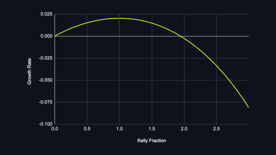
Note how the optimal growth rate is found at a Kelly fraction of 1 (the inflection point).

Based on the above, you’d be forgiven for thinking that all binary-outcome games should simply use the Kelly fraction at the maximum riskable amount from the LP’s counterparty.

There are disadvantages to doing so. The Kelly criterion is too aggressive for many people’s risk tolerance.

For example, in a stacked coin flip where the probability of a ‘Heads’ outcome is 60%, we’d get a Kelly fraction of 20% — working with the assumption that a win earns the played amount, while the loss loses it:

$$\frac{0.6}{1} - \frac{0.4}{1} = 0.2$$

To play with 20% of funds for a 60% chance of winning is a relatively high-risk endeavor – and, indeed, one that would likely be too risky for the average player to be comfortable with.

For every 24 coin flips, one can expect three ‘Tails’ in a row — resulting in a drawdown of 50%. This tracks, though: remember, the Kelly criterion aims to maximize growth rate versus minimizing the drawdown.

Since we cannot treat the liquidity pool’s funds as replenishable, full Kelly must be ruled out due to the risks of severe drawdowns like the above. Instead, full Kelly should serve as an upper bound on what can be reasonably risked, with 25-50% of that amount being considered reasonable. At launch, we begin with 10% before considering upping it to 25%.

Flipper

As mentioned earlier, Flipper emulates the mechanics of a coin flip — players select a side (Gold or Silver) and flip the coin. If their chosen side shows, they get 2x their played amount (before fees). If it doesn’t, they lose their played amount.

WIN PROBABILITY

In this game, the liquidity pool's probability of winning is 50% (or 0.5).

Let’s define the player’s played amount as 1. Should the liquidity pool lose, it should pay the user 1 (meaning that, as above, the user would leave with 2, or 2x their original entry). However, as the LP takes 1% (half of the total 2% fee) on its losses due to its fee, it actually pays out 0.96 to the player and 0.02 to future incentives — meaning the proportion of funds lost is 0.98.

In case of a win for the LP, it takes 1 (the player’s entire played amount).

contract

By inserting these calculated values into the Kelly Fraction for binary outcomes, we get a result of 0.0102040816. Since our probability and proportions remain constant, this Kelly Fraction was hard-coded into the smart contract.

Quantum

In Quantum, players aim to hit over or under a number. They can set their chance of being correct between 0.1-95%. Then, based on their chance, they’re assigned a multiplier.

WIN PROBABILITY

Probabilities and proportions of rounds will change based on user inputs. Here, we'll calculate the Kelly Criterion for the maximum and minimum multipliers.

Maximum multiplier

When the player selects the minimum chance of winning (0.1% or 0.001), their multiplier is 100/0.1 = a win of 1,000x.

Again, let’s call 1 the played funds for a given user. On a user win, the liquidity pool must pay 1,000x this amount — but since there's a 2% fee on the payout, they only receive 980x their played funds (10x goes towards the LP and 10x goes towards future incentives).

On an LP loss: the LP pays 989, as they do not pay for the user’s initial funds.

On an LP win: the LP wins 1. The probability of this happening is 1 - 0.001: 0.999, or 99.9%.

Inserting these numbers gives us:

x* = 0.999/989 - 0.001/1 = 0.00001011122

Minimum multiplier

Using the same logic outlined for the maximum multiplier, with a maximum chance of winning (95% or 0.95), we get the following equation:

x* = 0.05/0.04210526316 - 0.95/1 = 0.23749999994

contract

Because of the dynamic nature of the Kelly Fraction for Quantum, we opted to include an equation within the smart contract.

Multi-Outcome Games

Let’s follow similar steps to the Kelly Criterion for binary outcome games. Consider n possible outcomes, which each happen with probabilities p₁, p₂, … p_n, and payouts of M₁, M₂, … M_n. If our total funds start at B and we play with kB, then our expected value of the natural log of our total funds at the next step can be given by:

$$\sum_{i=1}^{n} p_{i} \ln((1 - k)B + kB + (M_{i} - 1)kB)$$

Factoring out B and simplifying produces:

$$\sum_{i=1}^{n}p_{i}ln(B(1+k(M_{i}-1)))$$

Using the multiplicative properties of logarithms, we can express this as:

$$\sum_{i=1}^{n}p_{i}ln(1+k(M_{i}-1))+ln(B)$$

Recall that the Kelly criterion can be found by taking the derivative and equating it to 0 to find the k value that produces the maximum growth rate:

$$\frac{d}{dk}(\sum_{i=1}^{n}p_{i}ln(1+k(M_{i}-1))+ln(B))=0$$

Therefore, the optimal fraction of total funds to be used as a counterparty is k, which is calculated by solving the following:

$$\sum_{i=1}^{n}\frac{p_{i}(M_{i}-1)}{(1+k(M_{i}-1))}=0$$

Where:

• n is the total number of outcomes
• p is the probability of a given outcome i
• M is the multiplier paid out to the play in given outcome i
• k is the Kelly fraction

note

To apply the equation from the LP's perspective, just treat the multipliers as negatives instead of positives.

Kelly Criterion Risks

Multiple concurrent entries at max Kelly

All games are susceptible to entry by multiple players concurrently. LPs are unable to update based on pending game results — so let’s explore the possible problems that may arise should many players enter at max Kelly.

A player’s max size is determined using the situation’s Kelly fraction. Should they win, the liquidity pool decreases, but the maximum playable size remains constant. This makes it possible for simultaneous rounds to be played above the Kelly fraction, as multiple successive wins lower the LP funds (thereby causing other rounds’ sizes to exceed 1x Kelly).

Continuing down this path, we could risk an entry’s size being so far above Kelly that it results in flat (or even negative) growth rates for the LP. The earlier diagram illustrates this principle for an amount of ~2x Kelly.

In games with small edges (as is the case on YOLO Games), growth rates tend to stagnate or turn negative at ~2x Kelly. However, higher fees can result in negative growth much sooner (e.g., at ~1.5x Kelly). You can see this in action by plotting the chart from the Binary-Outcome Games section and incrementally increasing p.

Let’s take a look at the difficulty required to hit 2x Kelly in our low-fee situation.

We’ll suppose that the LP’s capital starts at C, with a max payout of M (in the case of Flipper, this would be 1.98 — we consider the future incentives as a counterparty to the LP in this case , since we are focused on the LP’s risk), and a Kelly fraction of k. The max playable amount is C*k, while the maximum winnable amount is Ck(M-1). Such an event would reduce the initial LP to Ck(M-1).

Here’s the equation for the maximum playable amount:

$$MPA=Ck$$

Where:

• MPA is the maximum playable amount
• C is the LP’s capital
• k is the Kelly fraction

Here’s the equation for the maximum winnable amount:

$$MWA=MPA*(M-1)=Ck(M-1)$$

Where:

• MWA is the maximum winnable amount
• M is the max payout multiplier
• MPA is the maximum playable amount
• C is the LP’s capital
• k is the Kelly fraction

The maximum playable amount does not change over the course of multiple entries within the same round. However, in an ideal world, we would like for the Kelly fraction to re-compute the maximum playable amount after every round. To approach 2x Kelly, the player needs many consecutive wins in a row whilst entering with the maximum enterable amount. We can compute the bankroll after n wins using the following:

$$C_{n}=C(1-(M-1)k)^n$$

Where:

• C_n is the LP’s capital after n consecutive wins
• n is the number of consecutive wins
• M is the max payout multiplier
• C is the initial LP’s capital
• k is the Kelly fraction

If we substitute the LP after n wins equation (above) into the Maximum winnable amount equation , we can calculate the maximum winnable amount after n wins:

$$MWA_{n}=Ck(M-1)(1-(M-1)k)^n$$

Where:

• MWA_n is the maximum winnable amount after n wins
• n is the number of consecutive wins
• M is the max payout multiplier
• C is the initial LP’s capital
• k is the Kelly fraction

To identify the specific point where we risk >2x Kelly, we need to discover the number of games at which the maximum winnable amount (from no re-computation) is twice that of the maximum winnable amount (including re-computation).

Recall that:

• The maximum winnable amount from no re-computation is Ck(M - 1)
• The maximum winnable amount from re-computation is Ck(M - 1)(1 - (M - 1)*k)ⁿ

Sk(M - 1) can be canceled out, leaving us with the resulting equation, which determines the number of consecutive wins that must take place to reach 2x Kelly:

$$2=\frac{1}{(1-(M-1)*k)^n}$$

Where:

• M is the max payout multiplier
• k is the Kelly fraction
• n is the number of consecutive wins to reach 2x Kelly

Rearranging this equation gives us the following:

$$(1-(M-1)k)^{n}=0.5$$

To compute for n, we take the log/natural of both sides and rearrange:

$$n=\frac{ln(0.5)}{ln(1-(M-1)*k)}$$

So, with a maximum multiplier payout of 5 and a Kelly Fraction of 0.02, we would need 8.31 consecutive wins to reach 2x Kelly. Of course, this number must be an integer in practice, so we round it up to 9.

Alright, time to apply the equation to YOLO Games' suite. Since we apply the LP fee after the user has won, we need to replace M with (1-fee)*M in the aforementioned equation. Remember, we’re looking at this from the LP’s perspective — so we don’t include the portion of the fee that goes towards future incentives.

Flipper

Kelly Fraction	0.0102040816
Maximum Payout Multiplier	2

To reach 2x Kelly, we would need to lose ceil(ln(0.5)/ln((1-((2*0.99) - 1)*0.0102040816))) = 69 rounds in a row. The probability of this happening is 100*0.5⁶⁹ = ~1.6940659e-19%.

Quantum (Maximum possible multiplier)

Kelly Fraction	0.00001011122
Maximum Payout Multiplier	1000

To reach 2x Kelly, we would need to lose ceil(ln(0.5)/ln((1 - ((1000*0.99) -1)*0.00001011122))) = 69 rounds in a row. The probability of this happening is 100*0.001⁶⁹ = 1e-205%.

Quantum (Minimum possible multiplier)

Kelly Fraction	0.23749999994
Minimum Payout Multiplier	1.05

To reach 2x Kelly, we would need to lose ceil(ln(0.5)/ln((1 - ((1.05*0.99) - 1)*0.23749999994))) = 74 rounds in a row. This happens with a probability 1000.95⁷⁴ = 2.25%, but the player would have to risk kn = 17.575x the LP size.

LaserBlast (Maximum possible multiplier)

Kelly Fraction	0.000369
Maximum Payout Multiplier	1000.2

To reach 2x Kelly, we would need to lose ceil(ln(0.5)/ln((1 - ((1000.2*0.98) - 1)*0.000369))) = 2 rounds in a row. The probability of this happening is 100*(2*0.00153)² = 2.3409e-4%.